Optimizing time spent on numerically solving ODEs?

[ijustlovemath]

Sure. The base equation in questions is the Van Herpe ICU Minimal Model (two compartment insulin-glucose model):

Because there's a max() in dI1/dt, we do need to do some string parsing to decide on the actual F(X,t) that's being used (eg just -n(I1(t)-I_b) + FI/VI.

Additionally, FG and FI are time variant external inputs, so there's some more string parsing that has to be done. Finally, in our implementation of the model, we use a cubic spline interpolation technique to make n, VG, VI, and the constant in front of X(t) in dG/dt time variant. After all is said and done, the only non time-variant string is dX/dt.

The final equations look like this:

Here's the

[ijustlovemath]

Sorry, was editing the post with new info when it timed out. Here's the table of constants:

And for initial conditions, you can have G(0) = 200, X(0) = .01, I1(0) = 10, I2(0) = 0

[ijustlovemath]

Here's a quick python script you can run that uses RK4 on the base model (no time variant parameters, no exogenous inputs):

import time

def max(a,b):
    return a if a > b else b

''' 
Fourth order Runge-Kutta method in 4 dimensions.
Loops are unrolled from the RKN method for faster execution
'''
def RK4(_G, _X, _I1, _I2, dGdt, dXdt, dI1dt, dI2dt, hs):

	_G_1 = dGdt(_G, _X, _I1, _I2)*hs
	_X_1 = dXdt(_G, _X, _I1, _I2)*hs
	_I1_1 = dI1dt(_G, _X, _I1, _I2)*hs
	_I2_1 = dI2dt(_G, _X, _I1, _I2)*hs
    
	_G_k = _G + _G_1*0.5
	_X_k = _X + _X_1*0.5
	_I1_k = _I1 + _I1_1*0.5
	_I2_k = _I2 + _I2_1*0.5
    
	_G_2 = dGdt(_G_k, _X_k, _I1_k, _I2_k)*hs
	_X_2 = dXdt(_G_k, _X_k, _I1_k, _I2_k)*hs
	_I1_2 = dI1dt(_G_k, _X_k, _I1_k, _I2_k)*hs
	_I2_2 = dI2dt(_G_k, _X_k, _I1_k, _I2_k)*hs
    
	_G_k = _G + _G_2*0.5
	_X_k = _X + _X_2*0.5
	_I1_k = _I1 + _I1_2*0.5
	_I2_k = _I2 + _I2_2*0.5
    
	_G_3 = dGdt(_G_k, _X_k, _I1_k, _I2_k)*hs
	_X_3 = dXdt(_G_k, _X_k, _I1_k, _I2_k)*hs
	_I1_3 = dI1dt(_G_k, _X_k, _I1_k, _I2_k)*hs
	_I2_3 = dI2dt(_G_k, _X_k, _I1_k, _I2_k)*hs
    
	_G_k = _G + _G_3
	_X_k = _X + _X_3
	_I1_k = _I1 + _I1_3
	_I2_k = _I2 + _I2_3
    
	_G_4 = dGdt(_G_k, _X_k, _I1_k, _I2_k)*hs
	_X_4 = dXdt(_G_k, _X_k, _I1_k, _I2_k)*hs
	_I1_4 = dI1dt(_G_k, _X_k, _I1_k, _I2_k)*hs
	_I2_4 = dI2dt(_G_k, _X_k, _I1_k, _I2_k)*hs
    
	_G = _G + (_G_1 + 2.0*(_G_2 + _G_3) + _G_4)/6.0
	_X = _X + (_X_1 + 2.0*(_X_2 + _X_3) + _X_4)/6.0
	_I1 = _I1 + (_I1_1 + 2.0*(_I1_2 + _I1_3) + _I1_4)/6.0
	_I2 = _I2 + (_I2_1 + 2.0*(_I2_2 + _I2_3) + _I2_4)/6.0
    
	return _G, _X, _I1, _I2
    
# Exogenous flows would be communicated from LabVIEW, left 0 for now
FG_VG = 0 # mg/dL / min
FI_VI = 0 # uU/mL / min

P1_BASEVALUE = -1.31e-2
P2_BASEVALUE = -1.35e-2
P3_BASEVALUE = 2.90e-6

# Multipliers, varied using spline interpolation in application. Left constant here.
P1_MULT = 1
P2_MULT = 1
P3_MULT = 1

P1 = P1_MULT * P1_BASEVALUE
P2 = P2_MULT * P2_BASEVALUE
P3 = P3_MULT * P3_BASEVALUE

VHM_GB = 100 # mg/dL
VHM_IB = 10 # uU/mL
VHM_ALPHA = 3.11 # 1/min
VHM_H = 136 # mg/dL
VHM_N = .13 # 1/min
VHM_BETA = 1 # min
VHM_GAMMA = 5.36e-3 # ( uU/mL dL/mg ) / min^2

    
def dGdt(G,X,I1,I2):
    return (P1-X)*G-P1*VHM_GB+FG_VG
def dXdt(G,X,I1,I2):
    return P2*X+P3*(I1-VHM_IB)
def dI1dt(G,X,I1,I2):
    return VHM_ALPHA*max(0,I2)-VHM_N*(I1-VHM_IB)+FI_VI
def dI2dt(G,X,I1,I2):
    return VHM_BETA*VHM_GAMMA*(G-VHM_H)-VHM_N*I2
    
def runVHM():

    f = [dGdt, dXdt, dI1dt, dI2dt] # Function pointers
    x = [200, .01, 10, 0] # Initial conditions
    h = 1 # Time step of 1 minute
    
    __args = x+f+[h]
    
    N = 7200 # number of steps, translates to minutes of simulation with time step of 1.
    t0 = time.clock()
    for i in range(N):    
        __args[:4] = RK4(*__args)
        ''' <- Remove/add a hash before the block comment to toggle this block
        # Print solutions array as it comes, reduces performance by up to 100x
        print __args[:4]
        #'''
    t1 = time.clock()
    print 'Solution at end time:'
    print __args[:4]
    print 'Execution time: ' + str(1000*(t1-t0)/N) + 'ms'

runVHM()

It's fairly performant when you print solutions as they come, 4ms/iteration, with a massive 400% increase to .01ms/iteration when not printing anything. Although using a Shell Exec call takes anywhere from 100 to 300ms to get the output, so overall using this script would be a loss.

[johnsold]

Thanks for the equations.  I do not know Python so that code is not particularly helpful.

Can you post your VI so I can see how you coded the calls to RK4? That will save me from re-inventing the wheel and probably using different nomenclature.  I do not see any definition of the time-varying parameters: V(t), i_s(t), and i_h(t).

Lynn

[ijustlovemath]

Those are computed using the Cubic Spline Interpolation VIs; we design a curve, input it and the spline interpolates it. Here's the "core functionality" of the spline interpolation,

Although because of how much code you'd need for me to get individual curves sent, you can just leave those parameters set to 1.

[ijustlovemath]

Attached is (most of) the code you would probably need to look at my architecture. The VI specifically is under VHM/Models/VanHerpeModel/Run Model.vi

[ijustlovemath]

Did you get a chance to take a look?

[johnsold]

I started to take a look but have had several interruptions.  Multiple power outages due to thuderstorms, and having to do some actual work.  I will not have a chance to do much more until Wednesday afternoon or sometime on Thursday.

Lynn

[ijustlovemath]

Okay. Please let me know if I need to go into detail on anything within. Documentation is pretty sparse in this code, unfortunately.

[johnsold]

There are several classes missing so it is somewhat difficult to tell how everything fits together. I have a few suggestions although I cannot test them.

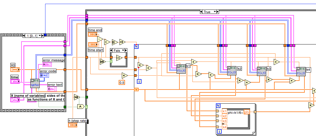
My focus is on the ODE solver using RK.  Part of the block diagram is shown below.

Note that the string array X and the time string connect to 5 subVIs.  When you look inside those subVIs, exactly the same decoding is done on those strings.

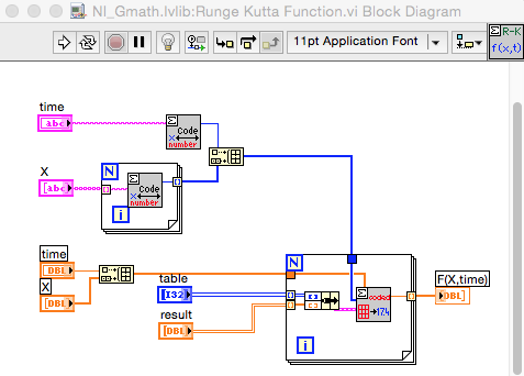
This is the BD of the RK Function.vi. The RK Syntax VI uses the same subVIs.

One suggestion is to create modified copies of the RK VIs which accept the integer arrays rather than strings. This way the strings only need to be converted once per call, or better, only when changed. Furthermore, look closely at the values passed to Decode.vi by your process. If you can do all the calculations on integers as opposed to a combination of strings and integers, it likely will be somewhat faster. Decode appears to process the ASCII values not the numeric values represented by the characters. 

The Formula Node in the RK Solver is a factor of 2 slower than the same calculation done with LV primitives for data arrays of 1000 elements or more. The differences are harder to determine for small arrays.

Some of the subVIs have a lot of coercion dots. These appear mostly on different size integers or integer-float conversions so the compiler probably does a pretty good job of eliminating any excess delays.  However, I would consider cleaning those up on any subVIs you modify for the other things I have mentioned.

If your data sets are small and the equations converge quickly you may not get much improvement. I think you could see noticeable speed up for large data sets and slow convergence.

Lynn